
Welcome to the first tutorial on Natural Language Processing (NLP) in the world of deep neural networks. Our goal is to enable everyone to grasp the knowledge in applying deep learning to NLP, no matter if you are a scientist, an engineer, a student, or anything else. We will guide you to go step-by-step with easy-to-follow examples using real data.
Outline
Let’s start with a simple example of predicting emotion. Consider the following two sentences:

Can you tell which one expresses sadness? Yes, the second one. This task is trivial for us, but how can we teach a machine to predict like humans?
A Brief Background on NLP
From Rules to Deep Learning Models
For long decades, practitioners in NLP focus on building hand-crafted rules and grammars for each language that are very tedious and laborious until statistical models are applied to NLP. Basically, those models are used to learn a function (or in layman terms, we call it mapping) between input and targets. Recently, deep learning models show significant progress in NLP, especially when open source deep learning frameworks, such as PyTorch, are available for academia and industry.
A simple naive solution for an NLP application is a keyword matching using rules. For example, in emotion classification tasks, we can collect words that represent happiness, and for sentences with those words, we can classify them as happy. But, is it the best we can do? Instead of checking word by word, we can train a model that accepts a sentence as input and predicts a label according to the semantic meaning of the input.
To show the difference between those methods, we will show you back the previous example!
By checking the lexical terms, we can easily fool our model to classify the second sentence as happy because it has won the jackpot phrase. If the model is able to understand the second sentence completely, then it is easy to notice the change of meaning after the second clause that makes that person feel sad because they didn’t win the jackpot.
Before we go to deep learning modeling with PyTorch, we will first explain briefly about the task categories in NLP.
Category of NLP Tasks
There are different tasks in Natural Language Processing. We can outline main categories of the NLP tasks as follow
- Text Classification
We aim to classify a text or document with a label class. Our example above is one of the examples. We predict an emotion label corresponding to the text. - Sequence Labeling
This is a task to predict a label for every token in the input. The most common task is Named Entity Recognition, the task to predict named entities in a given text input. - Language Generation
The task is to generate a sequence given a sequence as input. One of the examples is question answering task. Our model accepts a question and a context as input and generates an answer accordingly.
In this tutorial, we will show you an example of applying deep learning techniques on text classification. If you are new to deep learning, this will be a quickstart for you to start learning deep learning models using PyTorch.
Building a Model Using PyTorch
We’ll start simple. Let’s use the available pretrained model, and then fine-tune (train) the model again, to accommodate our example above. In this tutorial, we will use example in Indonesian language and we will show examples of using PyTorch for training a model based on the IndoNLU project.
PyTorch Framework
PyTorch is the best open source framework using Python and CUDA for deep learning based on the Torch library commonly used in research and production in natural language processing, computer vision, and speech processing. PyTorch is one of the most common deep learning frameworks used by researchers and industries. It is very intuitive for Numpy users as its core data structure, torch.Tensor, is pretty similar to numpy array. What difference is that torch.Tensor has the capability to be calculated in both CPU and CUDA, while in numpy it is not possible. It makes PyTorch a better tool for training deep learning models compared to Numpy. Another great thing is that PyTorch supports dynamic computation graphs and the network can be debugged and modified on the fly, unlike the static computation graph in Tensorflow. It makes PyTorch much more convenient to use for debugging because we can easily check the tensor during the execution of the code.
PyTorch can be installed and used in most operating systems via Anaconda or pip.
If you use Anaconda, PyTorch can be installed by executing the following command
conda install pytorch torchvision -c pytorch
If you use pip, PyTorch can be installed by executing the following command
pip install torch torchvision
To use the PyTorch library, simply import the PyTorch library
import torch
Sentiment Analysis Dataset
To add the benefit to your fun, let’s start with sentiment analysis, one of the most popular use cases yet easy to implement. Sentiment analysis is a natural language processing task to understand a sentiment within a body of text. In business, it is beneficial to automatically analyze customer review that is written i.e. in Twitter, Zomato, TripAdvisor, Facebook, Instagram, Qraved, and to understand the polarity of their review, whether it is a positive, negative, or a neutral review. As this kind of review dataset is included in one of the downstream tasks provided in the IndoNLU called SmSA along with all the needed resources, let’s begin our interesting project.
Data Preparation
Data preparation is one of the fundamental parts in modeling, it is even commonly said to take 60% of the time from the whole modeling pipeline. Fortunately, the tons of utilities provided by PyTorch and IndoNLU can simplify this process.
PyTorch provides a standardized way to prepare data for the model. It provides advanced features for data processing and to be able to utilize those features, we need to utilize 2 classes from torch.utils.data package, which are Dataset and DataLoader. Dataset is an abstract class that we need to extend in PyTorch, we will pass the dataset object into DataLoader class for further processing of the batch data. DataLoader is the heart of PyTorch data loading utility. It provides many functionalities for preparing batch data including different sampling methods, data parallelization, and even for distributed processing. To show how to implement Dataset and DataLoader in PyTorch, we are going to dig deeper into DocumentSentimentDataset and DocumentSentimentDataLoader classes from IndoNLU that can be found in the following link.
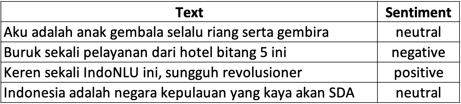
Before we begin with implementation, we need to know the format of our sentiment dataset. Our data is stored in tsv format and has two columns text and sentiment. Here are some examples of the dataset
Now, let’s start to prepare the pipeline. First, let’s import the required components
from torch.utils.data import Dataset, DataLoader
Next, we will implement the DocumentSentimentDataset class for loading our dataset. To make a fully functional DocumentSentimentDataset class, we need to at least define 3 different functions: __init__(self, ...), __getitem__(self, index), and __len__(self).
First, let’s define class and the __init__(self, ...) function
class DocumentSentimentDataset(Dataset):
    # Static constant variable (We need to have this part to comply with IndoNLU standard)
    LABEL2INDEX = {'positive': 0, 'neutral': 1, 'negative': 2} # Label string to index
    INDEX2LABEL = {0: 'positive', 1: 'neutral', 2: 'negative'} # Index to label string
    NUM_LABELS = 3 # Number of label

    def load_dataset(self, path):
        df = pd.read_csv(path, sep=’\t’, header=None) # Read tsv file with pandas
        df.columns = ['text','sentiment'] # Rename the columns
        df['sentiment'] = df['sentiment'].apply(lambda lab: self.LABEL2INDEX[lab]) # Convert string label into index
        return df

    def __init__(self, dataset_path, tokenizer, *args, **kwargs):
        self.data = self.load_dataset(dataset_path) # Load the tsv file

        # Assign the tokenizer for tokenization
        # here we use subword tokenizer from HuggingFace
        self.tokenizer = tokenizer
Now, we already have the data and the tokenizer defined in the __init__(self, ...) function. Next, let’s use it to __getitem__(self, index) and __len__(self) functions.
    def __getitem__(self, index):
        data = self.data.loc[index,:] # Taking data from a specific row from Pandas
        text, sentiment = data['text'], data['sentiment'] # Take text and sentiment from the row
        subwords = self.tokenizer.encode(text) # Tokenize the text with tokenizer

    # Return numpy array of subwords and label
        return np.array(subwords), np.array(sentiment), data['text']

    def __len__(self):
        return len(self.data)  # Return the length of the dataset
So, that’s it for the DocumentSentimentDataset. The full class definition is as follow:
class DocumentSentimentDataset(Dataset):
    # Static constant variable (We need to have this part to comply with IndoNLU standard)
    LABEL2INDEX = {'positive': 0, 'neutral': 1, 'negative': 2} # Label string to index
    INDEX2LABEL = {0: 'positive', 1: 'neutral', 2: 'negative'} # Index to label string
    NUM_LABELS = 3 # Number of label

    def load_dataset(self, path):
        df = pd.read_csv(path, sep=’\t’, header=None) # Read tsv file with pandas
        df.columns = ['text','sentiment'] # Rename the columns
        df['sentiment'] = df['sentiment'].apply(lambda lab: self.LABEL2INDEX[lab]) # Convert string label into index
        return df

    def __init__(self, dataset_path, tokenizer, no_special_token=False, *args, **kwargs):
        self.data = self.load_dataset(dataset_path) # Load the tsv file

        # Assign the tokenizer for tokenization
        # here we use subword tokenizer to convert text into subword
        self.tokenizer = tokenizer

    def __getitem__(self, index):
        data = self.data.loc[index,:] # Taking data from a specific row from Pandas
        text, sentiment = data['text'], data['sentiment'] # Take text and sentiment from the row
        subwords = self.tokenizer.encode(text) # Tokenize the text with tokenizer

    # Return numpy array of subwords and label
        return np.array(subwords), np.array(sentiment)

    def __len__(self):
        return len(self.data)  # Specify the length of the dataset
Notice that the dataset class returns subwords that can have different length for each index. In order to be fed to the model in batch, we need to standardize the length of the sequence by truncating the length and adding padding tokens. In this case we are going to implement the DocumentSentimentDataLoader class extending the PyTorch DataLoader.
In order to have the specified functionality, we need to override the collate_fn(self, batch) function from the DataLoader class. collate_fn() is a function that will be called after the dataloader collects a batch of data from the dataset. The argument batch consists of a list of data returned from the Dataset.__getitem__(). Our collate_fn(self, batch) function will receive list of subword and sentiment and spit out tuples of padded_subword, mask, and sentiment. mask is a variable that we use to prevent the model from considering the padding token as part of the input. To simplify, the visualization below shows the process of our collate_fn(self, batch) transform input subword into the padded subword and mask.
In the above visualization, 0 value means padding token. mask only consists of two values 0 and 1, where 0 means this token should be ignored by the model and 1 means this token should be considered by the model. OK, let’s now define our DocumentSentimentDataLoader
class DocumentSentimentDataLoader(DataLoader):
    def __init__(self, max_seq_len=512, *args, **kwargs):
        super(DocumentSentimentDataLoader, self).__init__(*args, **kwargs)
self.max_seq_len = max_seq_len # Assign max limit of the sequence length
        self.collate_fn = self._collate_fn # Assign the collate_fn function with our function

    def _collate_fn(self, batch):
        batch_size = len(batch) # Take the batch size
        max_seq_len = max(map(lambda x: len(x[0]), batch)) # Find maximum sequence length from the batch
        max_seq_len = min(self.max_seq_len, max_seq_len) # Compare with our defined limit

    # Create buffer for subword, mask, and sentiment labels, initialize all with 0
        subword_batch = np.zeros((batch_size, max_seq_len), dtype=np.int64)
        mask_batch = np.zeros((batch_size, max_seq_len), dtype=np.float32)
        sentiment_batch = np.zeros((batch_size, 1), dtype=np.int64)

    # Fill all of the buffer
        for i, (subwords, sentiment, raw_seq) in enumerate(batch):
            subwords = subwords[:max_seq_len]
            subword_batch[i,:len(subwords)] = subwords
            mask_batch[i,:len(subwords)] = 1
            sentiment_batch[i,0] = sentiment

    # Return the subword, mask, and sentiment data
        return subword_batch, mask_batch, sentiment_batch
Hooray!! We have implemented our DocumentSentimentDataLoader. Now let’s try to integrate this DocumentSentimentDataset and DocumentSentimentDataLoader. We can initialize our DocumentSentimentDataset and DocumentSentimentDataLoader in the following way:
dataset = DocumentSentimentDataset(‘./sentiment_analysis.csv’, tokenizer)
data_loader = DocumentSentimentDataLoader(dataset=dataset, max_seq_len=512, batch_size=32 num_workers=16, shuffle=True)
and then we can iterate our data loader by iterating it as follow
for (subword, mask, label) in data_loader:
    …
Pretty simple right? As you can see, in the DocumentSentimentDataLoader parameters, there are some additional parameters other than max_seq_len. The dataset parameter is a required parameter for DataLoader class, which is the data source used to fetch the data from. batch_size defines the number of data we will take per batch, num_workers defines the number of workers we want to use to fetch the data in parallel, and shuffle defines whether we want to take shuffle batch data or just fetch it in sequential order.
Ok, for the next section we are going to use our DocumentSentimentDataset and DocumentSentimentDataLoader for modeling purposes.
Model
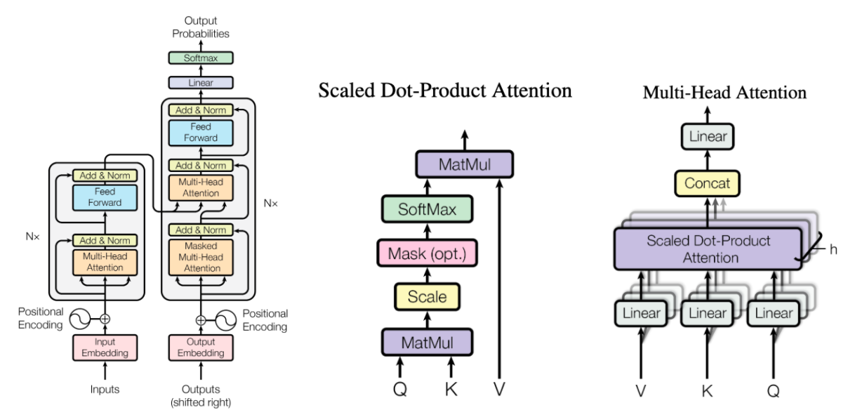
For our modeling purpose, we are going to use a very popular model in NLP called BERT. BERT is a very popular pre-trained contextualized language model that stands for Bidirectional Encoder Representations from Transformers. Just like what it says in its name, BERT makes use of transformers, the attention mechanism that takes contextual relations between words in a text into account. Before BERT, the most popular techniques were recurrent based models, which read the text input sequentially. What makes BERT better is that it removes the first order markov assumption and provides a self-attention mechanism.
There is an option to do modeling but not from scratch, that is to only tell the model to learn a little bit more from what it already knows. This kind of training is called fine-tuning. So here, we’re not doing the training from scratch, but rather, we will download the pretrained model from IndoNLU, specifically the indobenchmark/indobert-base-p1 model.
Now, let’s import the available pretrained model from the IndoNLU project that is hosted in the Hugging-Face platform. Thanks IndoNLU and Hugging-Face! For our sentiment analysis task, we will perform fine-tuning using the BertForSequenceClassification model class from HuggingFace transformers package.
from transformers import BertConfig, BertTokenizer, BertForSequenceClassification

tokenizer = BertTokenizer.from_pretrained("indobenchmark/indobert-base-p1")
config = BertConfig.from_pretrained("indobenchmark/indobert-base-p1")
Model = BertForSequenceClassification.from_pretrained("indobenchmark/indobert-base-p1", config=config)
Done! We now have the indobert-base-p1 tokenizer and model ready to be fine-tuned.
Training Phase
Here we are going to fine-tune the indobert-base-p1 model with our sentiment analysis dataset.
Another essential feature that PyTorch provides is the autograd package. So, before we jump into training the model, we first briefly welcome an autograd to join the team. Basically, what autograd does is to provide automatic differentiation for all operations that happened on Tensors. This framework automatically generates a computational graph that will be used in the backpropagation.
The finetuning training is done in these steps:
- Define an optimizer
Adamwith a small learning rate, usually below1e-3 - Enable the dropout regularization layer in the model by calling
model.train() - Enable the autograd computation by calling
torch.set_grad_enabled(True) - Iterate our data loader
train_loaderto getbatch_dataand pass it to the forward functionforward_sequence_classificationin the model. - Calculate the gradient by calling
loss.backward()to compute all the gradients automatically. This function is inherited by the autograd package. - Call
optimizer.step()to apply gradient update operation.’
We can see that the points above are coded in this below training script that we will use later for our finetuning.
optimizer = optim.Adam(model.parameters(), lr=3e-6)
model = model.cuda()

n_epochs = 5
for epoch in range(n_epochs):
    model.train()
    torch.set_grad_enabled(True)

    total_train_loss = 0
    list_hyp, list_label = [], []

    train_pbar = tqdm(train_loader, leave=True, total=len(train_loader))
    for i, batch_data in enumerate(train_pbar):
        # Forward model
        loss, batch_hyp, batch_label = forward_sequence_classification(model, batch_data[:-1], i2w=i2w, device='cuda')

        # Update model
        optimizer.zero_grad()
        loss.backward()
        optimizer.step()

        tr_loss = loss.item()
        total_train_loss = total_train_loss + tr_loss

        # Calculate metrics
        list_hyp += batch_hyp
        list_label += batch_label

        train_pbar.set_description("(Epoch {}) TRAIN LOSS:{:.4f} LR:{:.8f}".format((epoch+1),
            total_train_loss/(i+1), get_lr(optimizer)))

    # Calculate train metric
    metrics = document_sentiment_metrics_fn(list_hyp, list_label)
    print("(Epoch {}) TRAIN LOSS:{:.4f} {} LR:{:.8f}".format((epoch+1),
        total_train_loss/(i+1), metrics_to_string(metrics), get_lr(optimizer)))
The training script above uses the forward_sequence_classification function, as the forward function, and following is the snippet of the important parts of forward_sequence_classification function.
def forward_sequence_classification(model, batch_data, i2w, is_test=False, device='cpu', **kwargs):
    …
    if device == "cuda":
        subword_batch = subword_batch.cuda()
        mask_batch = mask_batch.cuda()
        token_type_batch = token_type_batch.cuda() if token_type_batch is not None else None
        label_batch = label_batch.cuda()

    # Forward model
    outputs = model(subword_batch, attention_mask=mask_batch, token_type_ids = token_type_batch, labels=label_batch)
        loss, logits = outputs[:2]
    …
    return loss, list_hyp, list_label
In both the training script and forward function above we leverage some of the pytorch capabilities, such as the easiness of switching the computation to CPU or GPU, the flexibilities of defining the loss function and computing the loss, and also the hassle-free gradient update by leveraging the autograd package to do the optimization and back propagation. Let’s add some more detail into the capabilities we are leveraging on.
Training Step
Here we are going to fine-tune the indobert-base-p1 model with our sentiment analysis dataset.
def train(model, train_loader, valid_loader, optimizer, forward_fn, metrics_fn, valid_criterion, i2w, n_epochs, evaluate_every=1, early_stop=3, step_size=1, gamma=0.5, model_dir="", exp_id=None):
    scheduler = StepLR(optimizer, step_size=step_size, gamma=gamma)

    best_val_metric = -100
    count_stop = 0

    for epoch in range(n_epochs):
        model.train()
        total_train_loss = 0
        list_hyp, list_label = [], []

        train_pbar = tqdm(iter(train_loader), leave=True, total=len(train_loader))
        for i, batch_data in enumerate(train_pbar):
            loss, batch_hyp, batch_label = forward_fn(model, batch_data[:-1], i2w=i2w, device=args['device'])

            optimizer.zero_grad()
            if args['fp16']:
                with amp.scale_loss(loss, optimizer) as scaled_loss:
                    scaled_loss.backward()
                torch.nn.utils.clip_grad_norm_(amp.master_params(optimizer), args['max_norm'])
            else:
                loss.backward()
                torch.nn.utils.clip_grad_norm_(model.parameters(), args['max_norm'])
            optimizer.step()

            tr_loss = loss.item()
            total_train_loss = total_train_loss + tr_loss

            # Calculate metrics
            list_hyp += batch_hyp
            list_label += batch_label

            train_pbar.set_description("(Epoch {}) TRAIN LOSS:{:.4f} LR:{:.8f}".format((epoch+1),
                total_train_loss/(i+1), get_lr(args, optimizer)))

        metrics = metrics_fn(list_hyp, list_label)
        print("(Epoch {}) TRAIN LOSS:{:.4f} {} LR:{:.8f}".format((epoch+1),
            total_train_loss/(i+1), metrics_to_string(metrics), get_lr(args, optimizer)))

        # Decay Learning Rate
        scheduler.step()

        # evaluate
        if ((epoch+1) % evaluate_every) == 0:
            val_loss, val_metrics = evaluate(model, valid_loader, forward_fn, metrics_fn, i2w, is_test=False)

            # Early stopping
            val_metric = val_metrics[valid_criterion]
            if best_val_metric < val_metric:
                best_val_metric = val_metric
                # save model
                if exp_id is not None:
                    torch.save(model.state_dict(), model_dir + "/best_model_" + str(exp_id) + ".th")
                else:
                    torch.save(model.state_dict(), model_dir + "/best_model.th")
                count_stop = 0
            else:
                count_stop += 1
                print("count stop:", count_stop)
                if count_stop == early_stop:
                    break
In both the training script and forward function above we leverage some of the pytorch capabilities, such as the easiness of switching the computation to CPU or GPU, the flexibilities of defining the loss function and computing the loss, and also the hassle-free gradient update by leveraging the autograd package to do the optimization and back propagation. Let’s add some more detail into the capabilities we are leveraging on.
CPU vs CUDA
model = model.cuda()
Training a million parameterized models like BERT on the CPU will take a vast amount of time. The linear algebra operations are done in parallel on the GPU and therefore you can achieve around 100x faster in training time. To cater for this need, PyTorch has prepared an easy way for us to move our tensor data typed variable to be computed either in CPU or GPU. This is done by accessing the method .cuda() or .cpu() in every tensor instantiated class and also the model, to move an object either to GPU memory from CPU memory, or vice versa.
Loss Function
    loss_fct = CrossEntropyLoss()
    total_loss = 0
    for i, (logit, num_label) in enumerate(zip(logits, self.num_labels)):
        label = labels[:,i]
        loss = loss_fct(logit.view(-1, num_label), label.view(-1))
        total_loss += loss
In PyTorch, we can build our own loss function or use loss function provided by the pytorch package. Building custom loss functions in Pytorch is not that hard actually, we just need to define a function that compares the output logits tensor with the label tensor and with that our loss function can have the same properties as the provided loss functions (automatically computed gradients, etc.). In our example here, we are using a provided loss function called CrossEntropyLoss(). Cross entropy loss is calculated by comparing how well the probability distribution output by Softmax matches the one-hot-encoded ground truth label of the data. We use this loss function in our sentiment analysis case because this loss fits perfectly to our needs as this is quantifying the model’s capability to distinguish the true sentiment from the possibility of the sentiments available in our data.
Optimizer and Back Propagation
optimizer = optim.Adam(model.parameters(), lr=5e-6)

optimizer.zero_grad()
loss.backward()
optimizer.step()
Initializing the optimizer needs us to explicitly tell it what parameters (tensors) of the model it should be updating. To do a back propagation, we only need to call .backward() on the loss Variable as this will start a process of backpropagation at the end loss and goes through all of its parents all the way to model inputs and output the gradient needed for backpropagation. Behind the curtain, while you’re called loss.backward(), gradients are “stored” by the tensors themselves (they have a grad and a requires_grad attributes). This is why, to do the backpropagation, optimizers don’t need to know anything about your loss. To update the gradient for all tensors in the model, we need to zero out all the previous grad from previous training by calling optimizer.zero_grad(), and then we need to call optimizer.step() as this will make the optimizer iterate over all parameters (tensors) it is supposed to update (requires_grad =True) and use their internally stored grad to update their values.
Evaluation Step
At each of the epoch training, we will evaluate the trained model performance. In the above finetuning training tutorial, we set the set_grad_enabled parameter as True, allowing all the gradients computed automatically when we call loss.backward(). In this evaluation phase, we don’t need that capability to be activated, and we don’t want to update any gradient parameters in any of the tensors. thus we set the set_grad_enabled parameter as False.
The fine tuning validation is done in these steps:
Enable the autograd computation by calling torch.set_grad_enabled(True).
Iterate our data loader valid_loader to get batch_data.
Pass it to the same forward function forward_sequence_classification in the model to output the model prediction.
Evaluate the predictions using sklearn functions that are provided in the document_sentiment_metrics_fn script, to output the accuracy, F1 score, recall, and precision.
We can see that the points above are coded in this below evaluation script that we will use for our fine tuning evaluation.
# Evaluate on validation
model.eval()
torch.set_grad_enabled(False)

total_loss, total_correct, total_labels = 0, 0, 0
list_hyp, list_label = [], []

pbar = tqdm(valid_loader, leave=True, total=len(valid_loader))
for i, batch_data in enumerate(pbar):
    batch_seq = batch_data[-1]
    loss, batch_hyp, batch_label = forward_sequence_classification(model, batch_data[:-1], i2w=i2w, device='cuda')

    # Calculate total loss
    valid_loss = loss.item()
    total_loss = total_loss + valid_loss

    # Calculate evaluation metrics
    list_hyp += batch_hyp
    list_label += batch_label
    metrics = document_sentiment_metrics_fn(list_hyp, list_label)

    pbar.set_description("VALID LOSS:{:.4f} {}".format(total_loss/(i+1), metrics_to_string(metrics)))

metrics = document_sentiment_metrics_fn(list_hyp, list_label)
print("(Epoch {}) VALID LOSS:{:.4f} {}".format((epoch+1),
    total_loss/(i+1), metrics_to_string(metrics)))
The evaluation script above uses the document_sentiment_metrics_fn function to do the mentioned accuracy, F1 score, recall, and precision metrics calculations, and the following is the snippet of it.
def document_sentiment_metrics_fn(list_hyp, list_label):
    metrics = {}
    metrics["ACC"] = accuracy_score(list_label, list_hyp)
    metrics["F1"] = f1_score(list_label, list_hyp, average='macro')
    metrics["REC"] = recall_score(list_label, list_hyp, average='macro')
    metrics["PRE"] = precision_score(list_label, list_hyp, average='macro')
    return metrics
This evaluation then concludes the whole modelling process. We hope you get a good result on your experiment and we hope you enjoyed our short but fun tutorial. If you have finished this tutorial, post your experiences and results in your facebook story. Inspire others to do the same by sharing this tutorial to other deep learning and NLP enthusiasts around the world!